July 2003Research:
Dances of the Planets
by Howard Arrington
The planets in the heavens move in exquisite orbital patterns,
dancing to the Music of the Cosmos. There is more mathematical
and geometric harmony than we realize. The idea for this
article is from a book Larry Pesavento shared with me. The
book, 'A Little Book of Coincidence' by John Martineau,
illustrates the orbital patterns and several of their geometrical
relationships. .
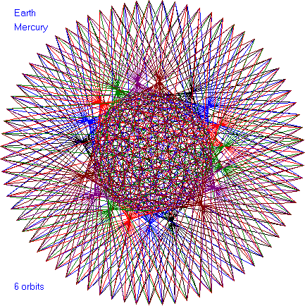
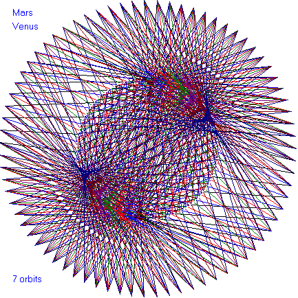
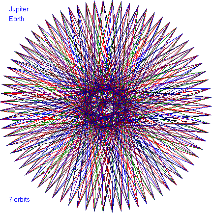
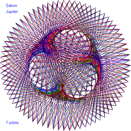
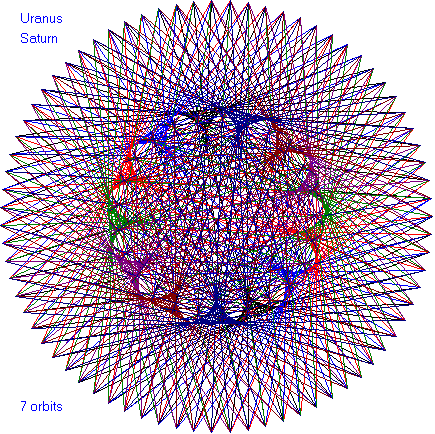
Take the orbits of any two planets and draw a line between the
two planet positions every few days. Because the inner planet
orbits faster than the outer planet, interesting patterns
evolve. Each planetary pairing has its own unique dance
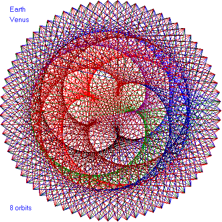
rhythm. For example, the Earth-Venus dance returns to the
original starting position after eight Earth years. Eight
Earth years equals thirteen Venus years. Note that 8 and 13
are members of the Fibonacci number series.
- Earth: 8 years * 365.256
days/year = 2,922.05
days
- Venus: 13 years * 224.701 days/year =
2,921.11 days (ie. 99.9%)
Watching the Earth-Venus dance for eight years creates this
beautiful five-petal flower with the Sun at the center. (5 is
another Fibonacci number.)
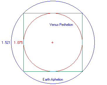
Another intriguing fact is the ratio between the Earth's outer
orbit and Venus's inner orbit is given by a square.
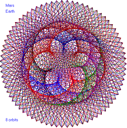
In the following dance patterns, the planet pairing is given and
the number of orbits of the outer planet. Enjoy these
beautiful patterns.
Let me share with you other facts about cosmic harmony. The
radius of the Moon compared to the Earth is three to eleven, ie.
3:11.
-
Radius of Moon = 1,080 miles = 3 x 360
-
Radius of Earth = 3,960 miles = 11 x 360
= 33 x 1 x 2 x 3 x 4 x 5
-
Radius of Earth plus Radius of Moon = 5,040
miles = 1 x 2 x 3 x 4 x 5 x 6 x 7 = 7 x 8 x 9 x 10
The ratio 3:11 is 27.3 percent, and the orbit of the
Moon takes 27.3 days. 27.3 days is also the average rotation
period of a sunspot. The closest : farthest distance ratio
that Venus and Mars each experiences in the Mars-Venus dance is
incredibly 3:11. The Earth orbits between them.
The sizes of the Moon and the Earth 'Square the
Circle' as shown in this illustration, which is drawn to
scale. The perimeters of the dotted square and the dotted
circle are the same length.
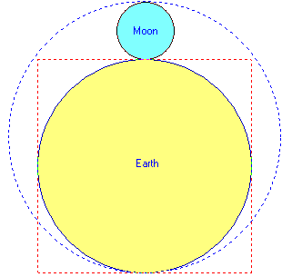
The perimeter of the dotted red square is 4 x Earth's
diameter = 4 x 7,920 miles = 31,680 miles.
The
circumference of the dotted blue circle is 2 pi x radius = 2 x 3.142
x 5040 miles = 31,667 miles. (ie. 99.9%)
ESPL:
Dances Program
by Howard Arrington
The dance patterns were drawn by the following ESPL program using
a chart window for the canvas. The chart bars and grid were
hidden so the canvas was blank. Edit the Planet1 and Planet2
variable values to select the planet pairing, with the planets
numbered beginning with Mercury = 1.
var {global variables}
i,c,Planet1,Planet2:
integer;
Planet1Year,Planet2Year: real;
Planet1Radius,Planet2Radius: real;
Interval,Orbits:
real;
yBottom,yCenter,xCenter: real;
a1,a2,a1Interval,a2Interval: real;
r,r1,r2,rStop:
real;
x1,y1,x2,y2: real;
function Year(i: integer):
real; {orbital period in days}
begin
if i=1 then Result:=87.969
else if i=2 then
Result:=224.701
else if i=3 then Result:=365.256
else if i=4 then Result:=686.980
else if i=5 then
Result:=4332.6
else if i=6 then Result:=10759.2
else if i=7 then Result:=30685
else if i=8 then
Result:=60190
else if i=9 then
Result:=90465;
end;
function Orbit(i: integer):
real; {mean orbit distance in 10^6
km}
begin
if i=1 then
Result:=57.91
else if i=2 then Result:=108.21
else if i=3 then Result:=149.60
else if i=4 then
Result:=227.92
else if i=5 then Result:=778.57
else if i=6 then Result:=1433.5
else if i=7 then
Result:=2872.46
else if i=8 then Result:=4495.1
else if i=9 then Result:=5869.7;
end;
function Name(i:
integer): string;
begin
if i=1 then
Result:='Mercury'
else if i=2 then
Result:='Venus'
else if i=3 then Result:='Earth'
else if i=4 then Result:='Mars'
else if i=5 then
Result:='Jupiter'
else if i=6 then
Result:='Saturn'
else if i=7 then
Result:='Uranus'
else if i=8 then
Result:='Neptune'
else if i=9 then
Result:='Pluto';
end;
begin {main program}
Planet1:= 3; {select outer planet}
Planet2:= 2; {select
inner planet}
Orbits := 8; {number of outer
rotations}
Planet1Year := Year(Planet1);
Planet2Year := Year(Planet2);
Planet1Radius :=
Orbit(Planet1);
Planet2Radius := Orbit(Planet2);
Interval := Planet1Year/75; {days}
FindWindow(eChart);
yBottom:=PriceToY(GetVariable(eScaleLow));
yCenter:=2+yBottom/2;
xCenter:=100+yCenter;
r1:=yCenter; {outer radius}
r2:=r1*Planet2Radius/Planet1Radius; {inner radius}
r:=0; rStop:=Planet1Year * Orbits;
a1:=0;
a1Interval:=2*pi*Interval/Planet1Year;
a2:=0;
a2Interval:=2*pi*Interval/Planet2Year;
SetPen(clBlue); {print labels}
TextOut(120,10,Name(Planet1));
TextOut(120,30,Name(Planet2));
TextOut(120,yBottom-30,inttostr(Orbits)+' orbits');
while r<rStop do begin
i:=trunc(r/interval/75); {use different color each
orbit}
if i=0 then
c:=clBlack
else if i=1 then
c:=clBlue
else if i=2 then
c:=clRed
else if i=3 then
c:=clGreen
else if i=4 then
c:=clPurple
else if i=5 then
c:=clMaroon
else if i=6 then
c:=clNavy
else if i=7 then
c:=clDkRed
else
c:=clOrange;
SetPen(c,1,eSolid,pmCopy);
a1:=a1-a1Interval;
{angle1}
a2:=a2-a2Interval;
{angle2}
x1:=r1*Cos(a1); y1:=r1*Sin(a1);
{convert polar to rectangular coordinates}
x2:=r2*Cos(a2); y2:=r2*Sin(a2);
MoveToLineTo(x1+xCenter,y1+yCenter,x2+xCenter,y2+yCenter);
{draw line}
r:=r+Interval; {move around
outer circumference}
end;
end;
Research:
The Art of Optimizing
by
Howard Arrington
I recently designed a trading system in Ensign Windows using a
few Study Alerts to implement the Buy, Sell, and Exit rules.
The system was simple wherein it used a Parabolic Stop study to
determine market direction, and would buy retracements in an uptrend
and sell retracements in a downtrend. The system would exit
any position when a scalp objective had been achieved, or when a
protective stop was touched.
This trading system had 4 adjustable parameters:
Parabolic Acceleration Rate, Stop Size, Scalp Size, and Retracement
Size. After several quick guesses for each parameter's
setting, the test results implied that the system was most sensitive
to the parameters in the order as listed. It seemed
logical that the parameters should be optimized in the order of
their sensitivity from most sensitive to least
sensitive. Therefore, the first step of optimization was
to pick 'in-the-ballpark' parameter values for the other parameters
while the Parabolic Acceleration Rate parameter was adjusted in
small increments.
The training data set consisted of 10 consecutive days of day
session 2-minute bars for the Emini futures contract.
These 10 days included a variety of market conditions such as
trending days, sideways choppy days, several large opening gaps up
and down, and occasional periods of wild volatility. The
10-day period seemed sufficient for the purpose of finding
appropriate parameter values. All results are for trading 1
Emini contract with no deduction for commissions or slippage.
To optimize the Parabolic Acceleration Rate, values were adjusted
from 0.35 through 0.65 in increments of 0.05 while the other
parameters were fixed at these values:
Stop Size = 6 points Scalp
Size = 7 points
Retracement Size = 2 points. The worst
results were $812 profit on 44 trades using the 0.35
setting. The best results were $3887 profit on 49 trades
at the 0.50 setting.
The protective Stop Size was optimized by testing values from 1
point through 10 points in 1 point increments. Scalp
Size and Retracement Size remain unchanged. The Parabolic
parameter used the 0.50 setting. The worst results were $3337
profit on 54 trades using the 3 point Stop. The best results
were $3900 on 49 trades using a 7 point Stop.
The Scalp Size was optimized by testing values from 1 point
through 10 points in 1 point increments. The other parameters
used were these values: Retracement Size = 2
points Stop Size = 7
points Parabolic =
0.50. The worst results were $2312 profit on
100 trades using a 1 point scalp objective. The best results
were $4500 on 58 trades using a 5 point scalp objective.
This result would lend support to Larry Pesavento's claim that a
natural harmonic swing size of 5.40 points exists in the S&P and
ES markets.
Finally, the Retracement Size parameter was optimized by testing
values from 1 point through 5 points in half point increments.
The worst results were $62 profit on 5 trades using a 5 point
retracement requirement. The best results were $4775
profit on 64 trades using a 1.50 point retracement size.
The following example shows the trading system in operation using
the optimized parameter values.
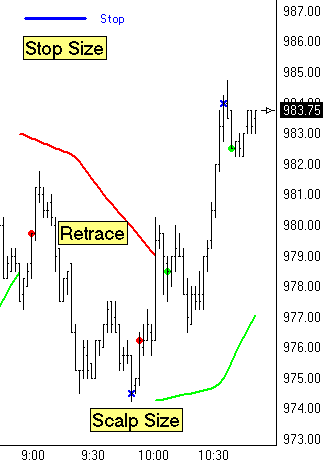
Just prior to 9:00 a downward move in the market
reversed the Parabolic Stop study to a down trend as indicated by
the falling Red curve. The retrace that followed
exceeded the Retracement Size requirement of 1.50 points, so the
system sold Short and used as its fill price the Close of the bar
marked by the 1st Red dot. The Scalp objective of 5
points was achieved 50 minutes later so the system exited this Short
trade and used as its fill price the Close of the bar marked by the
Blue X. During this Short trade, the protective Stop was
7 points away from the entry price and marked on the chart with a
horizontal blue line.
After this successful scalp trade, the retracement
requirement was satisfied again while the Parabolic was still in a
down trend. The system sold Short a 2nd time at the 2nd Red
dot near 10:00. The market did not continue lower as
expected, but rose to trigger a reversal of the Parabolic Stop to an
uptrend indicated by the rising Green curve. A retracement in
the uptrend initiated a Buy signal. Therefore, the Short trade
was closed out at a loss and a Long trade was initiated using as its
fill price the Close of the bar marked by the 1st Green
dot. This long trade was successful and existed at the 5
point scalp objective marked by the 2nd Blue X near the swing
top. A 2nd long trade was initiated on the retracement
marked by the 2nd Green dot.
Once optimized values were determined for each of the parameters,
a quick recheck was done of each of the parameters to see if they
had shifted in either direction now that better parameters were
known for the others. The values determined above
remained the optimal settings. Perhaps it was just
coincidence, and perhaps it was because the initial
'in-the-ballpark' values were close to the optimized
values. The system has been tuned to optimal performance
(at least for the past 10 days) using these values:
Parabolic = 0.50 Stop Size = 7
points Scalp Size = 5
points Retracement Size = 1.50 points.
The system was run the next day with 3 successful scalps and 2
losses. The net for the 5 trades added another $385 to the
total profit.
The next step in the evolution of the system was to examine each
of the 64 trades that generated the $4775 profit in the 10-day
trading data set. The general statistics showed that there
were 37 winners (58%) and 27 losers (42%). While some of
the parameter combinations generated win/loss percentages as
favorable as 80/20, the profitability was always lower because fewer
trades were taken. For some traders, that would be a desirable
characteristic. For this optimized system the Average Winner
was $180 and the Average Loser was $70. Both of these
numbers are very good. The Average Trade Profit was $75, which
is sufficient to pay for a round trip commission and tolerate a tick
slippage.
The examination of the trades showed that 7 times the system was
in a position at market close and carried the position
overnight. The effect of holding the position overnight was
surprisingly favorable with 6 winners and 1 loser with these point
totals: +10, +7, +2, +7, +3, +2, and -7 points for the only
loser. Thus the overnight effect added 24 points or $1200 to
the overall system profitability. This was an unexpected
result, but the 10-day data set included several gap openings, and
the system happened to be on the right side of those gaps 6 out of 7
times.
The system was modified to exit any position at market close so
no position was held overnight. This would be a characteristic
preferred by day traders, and the overall system performance was
less profitable as expected.
The overnight effect was intriguing and generated the need to
test that idea as a separate trading system. So, in a matter
of minutes, Study Alerts were configured to Buy the Close of the day
session if the Parabolic Stop was Long, and Sell the Close of the
day session if the Parabolic Stop was Short. This simple
system would exit on the Close of the first 2 minute bar of the
following day's day session open. That's it.
One trade per day, either buying or selling the last bar of the day
session and exiting the following day on the first bar of the next
day session. The system had a $2300 profit on 9 trades for the
10-days in the test data set.
Now, do any of my ideas and numbers represent the 'Holy Grail' of
trading systems. Absolutely not. The purpose of
this article was to walk system designers through the thought
process of how parameters that define a trading system might be
adjusted a maximize a system's performance across a test data
set. Some may wish to maximize the win/loss ratio, while
others (myself included) prefer to maximize the total dollar profit
as long as the trading frequency is not excessive. For my
simple system, 64 trades in 10 days is a trade frequency of 5 to 8
trades per day session, which is realistic for a scalping system.
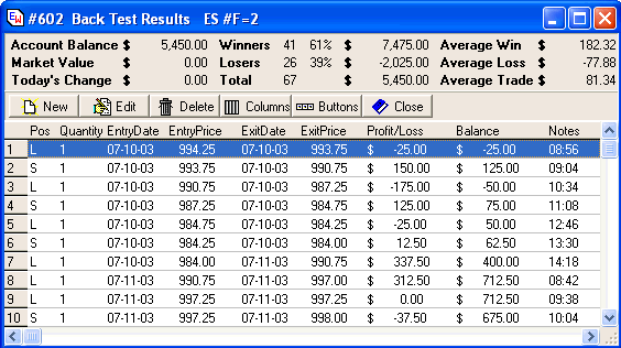
Here is a example Trade Ledger that logs the details of each of
the trades taken by the system. The form shows some of the
statistics used to evaluate whether one set of parameters is better
or worse than another set of parameters. The Notes field shows
the Time of day the trade was executed.
Note: If you have Ensign Windows and wish to experiment
with this trading system, it can be downloaded from the Ensign web
site using the Internet Services form in Ensign Windows. Open
the Internet Services form and click the Upgrade tab. Click
the Connect button. Then select the Template bullet and the
July24th name in the template list. Click the Download
button to put the system on your computer. Enjoy.
Disclaimer: Past performance is no guarantee of
equivalent future performance. All results in this article are
hypothetical and do not include commissions and slippage
penalties. This system was optimized for a particular 10-day
period of time and designed with the benefit of
hindsight. Results from the system with any other data
set, past or future, will in all likelihood be less
impressive. No representation is being made that any account
will or is likely to achieve the profits or losses similar to those
shown. This trading system is being shared solely for its
educational value and should not be a basis for placing actual
trades. |